To begin our analysis, we obtained the ‘Dissemination Block’ (DB) layer and DMTI Route Logistics ‘Streets’ layer, along with the ‘Vancouver Fire Halls’ layer from the UBC Geography Department server. In order to locate the fire halls for the other municipalities, we created an Address Locator using US Dual Ranges. Once this was created, we simply used each city’s website to obtain the fire hall addresses and used the ‘Find’ tool in Arc to geocode the fire halls into our map.

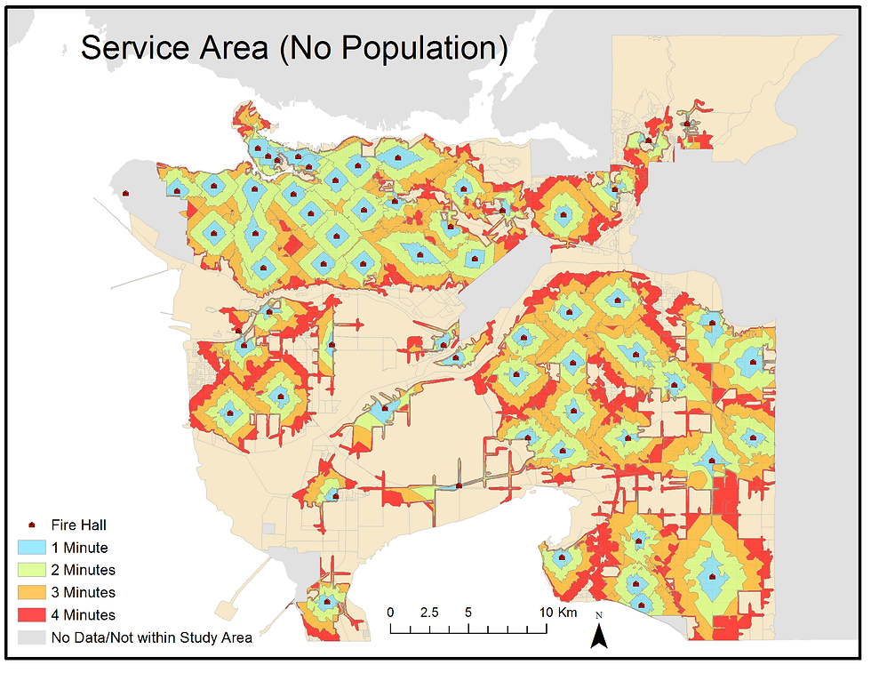
       To create Service Area 1, we then created a Network Dataset using the ‘Streets’ file which contained the travel times for each segment of road within its attribute table. We then created service areas originating from each fire hall point location based on these travel times. Service Area 1 does not take into account population density and how this might affect traffic congestion and ultimately the response times.

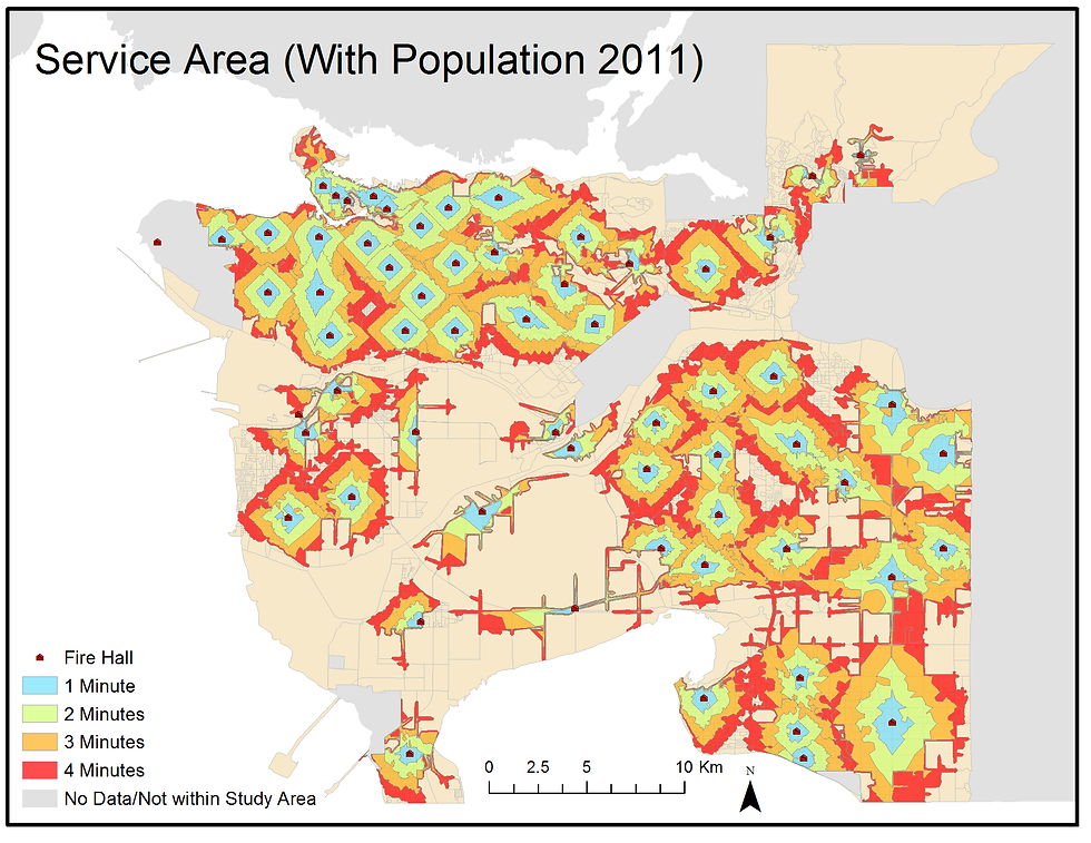
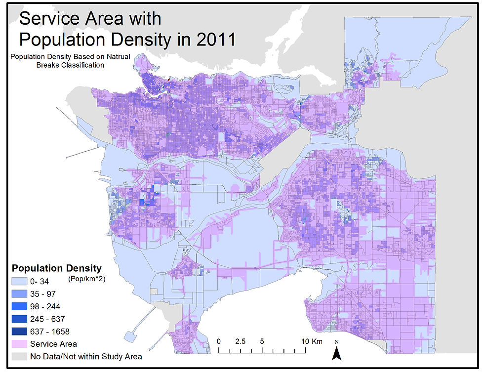
       To create Service Area 2, we first had to create a population density map. To do this we used the ‘Feature to Point’ tool to change the DB polygons into points and then created a point density map by using the ‘Point Density’ tool. We then implemented the ‘Feature to Point’ tool on the ‘Streets’ layer which created points on the centroid of each line segment. This gave us a point density map as well as street points and by using the ‘Extract Value to Point’ tool, we were able to create a population density map in raster form. We then reclassified the population densities into low (less than 3,000 people per square kilometer), medium (3,000 to 20,000 people per square kilometer) and high (more than 20,000 people per square kilometer) and then joined this table with the ‘Streets’ attribute table. We then recalculated the travel times using the field calculator. Travel times were not changed for areas in the low density class. Travel times were multiplied by 1.25 for areas in the medium density class and travel times were multiplied by 1.5 for areas in the high density class. Demographia (n.d.) is what we based our classes and multiplication factors on. With these new travel times taking into account population densities in 2011, we created a new Network Dataset and again using the ‘Network Analyst’ tool, we created Service Area 2.

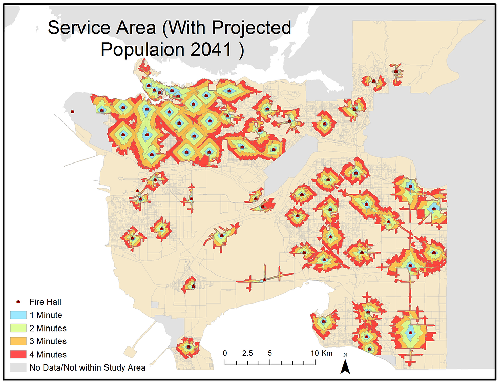
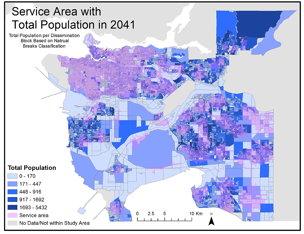
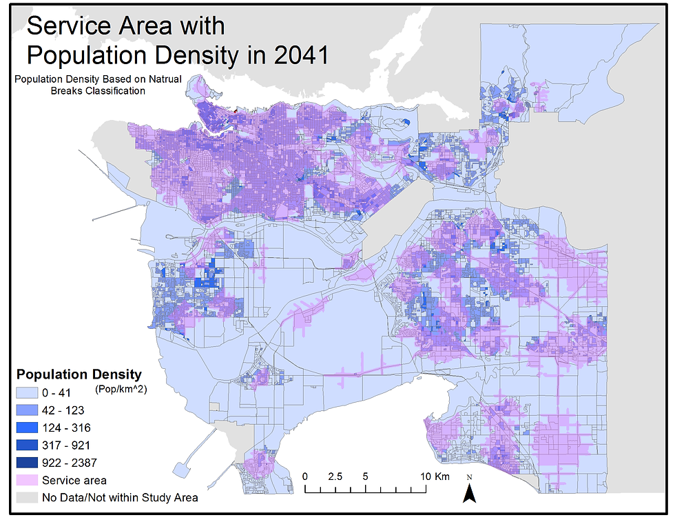
       To create Service Area 3 we simply had to recalculate the travel times again but this time taking into account the projected population in 2041 according to Metro 2040 (2009) projections. With these projected population numbers and the population numbers from 2011, we easily calculated the per cent change and from this we calculated new travel times following the method of Brinklow et al., (2006) which designates that a per cent change in population of x will constitute the travel times being multiplied by 1.x. With these new travel times taking into account projected 2041 population counts, a third Network Dataset was created and from this, Service Area 3.

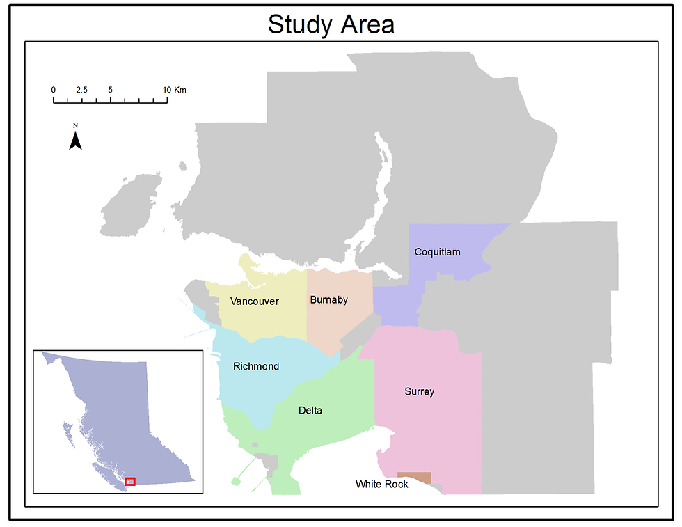
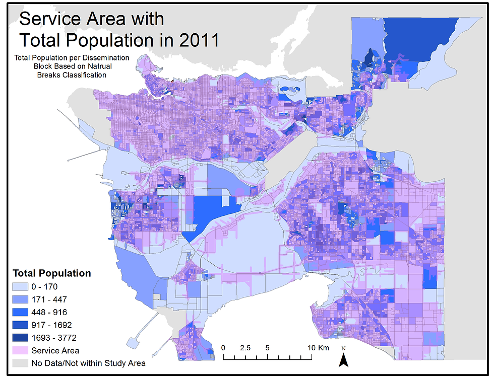
       Once all three service areas were created we then wanted to calculate the number of people that fall outside of the four-minute response time in both scenarios. To do this, we selected our seven municipalities from the ‘DB’ layer using ‘Select by Attributes’ and then exported this to a new layer showing only our cities of interest. We then simply eliminated Service Area 2 and Service Area 3 from the ‘Seven Cities’ layer using the ‘Erase’ tool and then created two summary tables, one for 2011 and one for 2041, that were summarized by population and this gave us our final numbers. For more details on our calculations and final numbers, see our Discussion section.